一、singleR
1. 总体代码
#第二种方法用SingleR鉴定细胞类型

###下载好数据库后,把ref_Human_all.Rdata加载到环境中,这样算是对数据库的加载,就可以按照singler的算法来对细胞亚群进行定义了。
load("~/ref_Human_all.RData")
###我们可以看到在环境中多了一个叫ref_Human_all的文件 大小为113mb  这个就是数据库
####然后我们把环境中的ref_Human_all赋值与refdata
refdata <- ref_Human_all
###把rna的转录表达数据提取
?GetAssayData
testdata <- GetAssayData(scRNA_harmony, slot="data")
###把scRNA数据中的seurat_clusters提取出来,注意这里是因子类型的
clusters <- scRNA_harmony@meta.data$seurat_clusters
###开始用singler分析
cellpred <- SingleR(test = testdata, ref = refdata, labels = refdata$label.main,
                    method = "cluster", clusters = clusters,
                    assay.type.test = "logcounts", assay.type.ref = "logcounts")
###制作细胞类型的注释文件
celltype = data.frame(ClusterID=rownames(cellpred), celltype=cellpred$labels, stringsAsFactors = FALSE)
###保存一下
write.csv(celltype,"celltype_singleR.csv",row.names = FALSE)
##把singler的注释写到metadata中 有两种方法
###方法一
scRNA_harmony@meta.data$celltype <- NA
celltype$ClusterID <- as.integer(celltype$ClusterID)
scRNA_harmony@meta.data$seurat_clusters1 <- scRNA_harmony@meta.data$seurat_clusters
scRNA_harmony@meta.data$seurat_clusters1 <- as.integer(scRNA_harmony@meta.data$seurat_clusters1)
?which
for(i in 1:nrow(celltype)){
  scRNA_harmony@meta.data[which(scRNA_harmony@meta.data$seurat_clusters == celltype$ClusterID[i]),'celltype'] <- celltype$celltype[i]
}

###因为我把singler的注释加载到metadata中时候,命名的名字叫celltype,所以画图时候,group.by="celltype"
DimPlot(scRNA_harmony, group.by="celltype", label=T, label.size=5)
###方法二:
celltype = data.frame(ClusterID=rownames(cellpred), celltype=cellpred$labels, stringsAsFactors = F)
scRNA_harmony@meta.data$singleR=celltype[match(clusters,celltype$ClusterID),'celltype']
###因为我把singler的注释加载到metadata中时候,命名的名字叫singleR,所以画图时候,group.by="singleR"
DimPlot(scRNA_harmony, group.by="singleR", label=T, label.size=5)

#####使用来自scRNAseq包中的两个人类胰腺数据集。目的是使用一个预先标记好的数据集对另一个未标记的数据集进行细胞类型注释。
#首先,我们使用Muraro et al.(2016)的数据作为我们的参考数据集。
BiocManager::install("scRNAseq")
library(scRNAseq)
sceM <- MuraroPancreasData()
sceM.1 <- sceM[,!is.na(sceM$label)]
BiocManager::install("scater")
library(scater)
sceM.1 <- logNormCounts(sceM.1)
##接下来,我们使用Grun et al.(2016)的数据作为测试数据集。
##有时候可能网速不好哟
sceG <- GrunPancreasData()

# Remove libraries with no counts.
sceG <- sceG[,colSums(counts(sceG)) > 0]
sceG <- logNormCounts(sceG)
#为了加快分析的速度,我们挑选前200个细胞进行分析。
sceG <- sceG[,1:500]
# 使用SingleR函数进行细胞类型注释,并指定de.method="wilcox"检测方法
pred.grun <- SingleR(test=sceG, ref=sceM.1, labels=sceM.1$label, de.method="wilcox")

# 查看细胞类型注释的预测结果
table(pred.grun$labels)

####注释结果诊断
###1.基于scores within cells
### Annotation diagnostics
plotScoreHeatmap(pred.grun)
# 基于 per-cell “deltas”诊断,Delta值低,说明注释结果不是很明确
plotDeltaDistribution(pred.hesc, ncol = 3)
2. GetAssayData()
Assays对象的通用访问函数和设置函数。GetAssayData 可用于从任何表达式矩阵(如 "counts"、"data "或 "scale.data")中提取信息。SetAssayData 可用于替换其中一个表达式矩阵
3. SingleR()
根据同一特征空间中已标注的参考数据集,返回测试数据集中每个单元格的最佳注释。SingleR是一种用于单细胞RNA测序(scRNAseq)数据的自动标注方法。给定一个具有已知标签的参考样本集(单细胞或批量),它根据与参考的相似性对来自测试数据集的新单元格进行标记。因此,对于参考数据集,手动解释集群和定义标记基因的负担只需要做一次,并且这种生物知识可以以自动的方式传播到新的数据集。singleR自带的7个参考数据集,其中5个是人类数据,2个是小鼠的数据:
- BlueprintEncodeData Blueprint (Martens and Stunnenberg 2013) and Encode (The ENCODE Project Consortium 2012) (人)
- DatabaseImmuneCellExpressionData The Database for Immune Cell Expression(/eQTLs/Epigenomics)(Schmiedel et al. 2018)(人)
- HumanPrimaryCellAtlasData the Human Primary Cell Atlas (Mabbott et al. 2013)(人)
- MonacoImmuneData, Monaco Immune Cell Data - GSE107011 (Monaco et al. 2019)(人)
- NovershternHematopoieticData Novershtern Hematopoietic Cell Data - GSE24759(人)
- ImmGenData the murine ImmGen (Heng et al. 2008) (鼠)
- MouseRNAseqData a collection of mouse data sets downloaded from GEO (Benayoun et al. 2019).(鼠)
4.plotScoreHeatmap()
plotScoreHeatmap显示所有引用细胞类型上所有细胞的得分,这允许用户检查数据集中预测细胞类型的可信度。每个类群/细胞的实际分配标签显示在顶部的颜色栏中。关键点是检查分数(scores)在每个类群/细胞中的分布情况。理想情况下,每个类群/细胞(即热图的列)应该有一个明显大于其他细胞的分数,这表明它明确地分配给了单个标签。
二、Garnett
从单细胞表达数据中实现自动细胞类型分类的软件包。使用人工定义的marker基因选择细胞,基于这些细胞使用弹性网络回归的机器学习算法训练分类器。
自己训练分类器:
1.制作符合garnett格式要求的定义细胞类型的marker基因文本文件(marker file);
2.使用单细胞数据创建monocle3的CDS数据对象;
3.将两种文件输入garnett,对marker基因进行打分,根据评分优化marker file;
4.将优化后的marker file和cds object输入garnett训练分类器。
BiocManager::install(c('BiocGenerics', 'DelayedArray', 'DelayedMatrixStats',
                       'limma', 'S4Vectors', 'SingleCellExperiment',"batchelor",
                       'SummarizedExperiment'))

# 安装monocle3
devtools::install_github('cole-trapnell-lab/monocle3')
library(monocle3)
## 然后安装常用的人和小鼠的基因信息数据库
BiocManager::install(c('org.Hs.eg.db', 'org.Mm.eg.db'))

## 最后安装garnett
devtools::install_github("cole-trapnell-lab/garnett", ref="monocle3")
library(garnett)

download.file(url="https://cole-trapnell-lab.github.io/garnett/marker_files/hsPBMC_markers.txt",
              destfile = "hsPBMC_markers.txt")

download.file(url="https://cf.10xgenomics.com/samples/cell-exp/3.0.2/5k_pbmc_v3_nextgem/5k_pbmc_v3_nextgem_filtered_feature_bc_matrix.h5",
              destfile = "pbmc.h5")

download.file(url="https://cole-trapnell-lab.github.io/garnett/classifiers/hsPBMC_20191017.RDS",
              destfile = "hsPBMC.rds")
getwd()
###

## 创建seurat对象并降维聚类

load("C:/shangke/lession11/scRNA_harmony.rdata")
pbmc <- scRNA_harmony
cell=colnames(scRNA_harmony)
pbmc=pbmc[,cell]
pbmc <- SCTransform(pbmc)
pbmc <- RunPCA(pbmc, verbose = F)
ElbowPlot(pbmc)
pc.num=1:15
pbmc <- pbmc %>% RunTSNE(dims=pc.num) %>% RunUMAP(dims=pc.num) %>%
  FindNeighbors(dims = pc.num) %>% FindClusters(resolution=0.8)

## 创建CDS对象
data <- GetAssayData(pbmc, assay = 'RNA', slot = 'counts')
cell_metadata <- pbmc@meta.data
gene_annotation <- data.frame(gene_short_name = rownames(data))
?data.frame
rownames(gene_annotation) <- rownames(data)
cds <- new_cell_data_set(data,
                         cell_metadata = cell_metadata,
                         gene_metadata = gene_annotation)
?new_cell_data_set
#preprocess_cds函数相当于seurat中NormalizeData+ScaleData+RunPCA
cds <- preprocess_cds(cds, num_dim = 30)

## 演示利用marker file训练分类器
# 对marker file中marker基因评分
library(org.Hs.eg.db)
marker_check <- check_markers(cds, "hsPBMC_markers.txt",
                              db=org.Hs.eg.db,
                              cds_gene_id_type = "SYMBOL",
                              marker_file_gene_id_type = "SYMBOL")
?check_markers
plot_markers(marker_check)

# 使用marker file和cds对象训练分类器
pbmc_classifier <- train_cell_classifier(cds = cds,
                                         marker_file = "hsPBMC_markers.txt",
                                         db=org.Hs.eg.db,
                                         cds_gene_id_type = "SYMBOL",
                                         num_unknown = 50,
                                         marker_file_gene_id_type = "SYMBOL")
?train_cell_classifier
saveRDS(pbmc_classifier, "my_classifier.rds")

#查看分类器最后选择的根节点基因,注意markerfile的基因都会在其中
feature_genes_root <- get_feature_genes(pbmc_classifier, node ="root", db= org.Hs.eg.db,
                                       convert_ids = TRUE)
?get_feature_genes
head(feature_genes_root)

#使用garnett官网训练好的分类器预测数据。
download.file(url="https://cole-trapnell-lab.github.io/garnett/classifiers/hsPBMC_20191017.RDS",
              destfile = "hsPBMC.rds", mode = "wb")

hsPBMC <- readRDS("hsPBMC.rds")
?pData
pData(cds)
pData(cds)$garnett_cluster <- pData(cds)$seurat_clusters
cds <- classify_cells(cds,
                      pbmc_classifier,
                      db = org.Hs.eg.db,
                      cluster_extend = TRUE,
                      cds_gene_id_type = "SYMBOL")

# 提取分类结果
cds.meta <- subset(pData(cds), select = c("cell_type", "cluster_ext_type")) %>% as.data.frame()
## 将结果返回给seurat对象
?AddMetaData
pbmc <- AddMetaData(pbmc, metadata = cds.meta)

tsne <- as.data.frame(pbmc@reductions[["tsne"]]@cell.embeddings)
data <-  as.data.frame(pData(cds))
data_umap <- merge(data,tsne,by=0)
colnames(data_umap)
qplot(tSNE_1, tSNE_2, color = cell_type, data = data_umap) + theme_bw()
?qplot

qplot(tSNE_1, tSNE_2, color = cluster_ext_type, data = data_umap, labels= T) + theme_bw()
##上图中第一个图显示了Garnett的细胞类型分配,第二张图显示了Garnett的cluster群扩展类型分配。
1.new_cell_data_set()
new_cell_data_set ( ):从头创建CDS对象并预处理数据,创建了一个全新的对象,这样很繁琐,还要再做一次降维聚类分群。因为我们导入了seurat对象里的表达矩阵,meta信息和genelist,所以这个cds是没有进行降维聚类等操作,导致后面的拟时序分析是做不了的,官网上说拟时序分析是基于低维度,所以必须对cds进行降维聚类分群。
new_cell_data_set(expression_data, cell_metadata = NULL, gene_metadata = NULL)
Arguments
expression_data
expression data matrix for an experiment, can be a sparseMatrix.

cell_metadata
data frame containing attributes of individual cells, where row.names(cell_metadata) = colnames(expression_data).

gene_metadata
data frame containing attributes of features (e.g. genes), where row.names(gene_metadata) = row.names(expression_data).
as.cell_data_set ( ): 直接读入经过Seurat上游处理(SCTransform、RunPCA、RunUMAP、FindNeighbors、FindClusters)后的obj创建rds对象,不用再进行预处理(preprocess_cds)和降维(reduce_dimension)步骤。
2.marker文件准备
1.
>开头的细胞类型行;
2.expressed:开头行,后面跟定义细胞类型的marker基因。基因之间使用,分隔。
可选以下几行的附加信息:
1.not expressed:开头行,后面跟定义细胞类型的负选marker基因。例如CD4+T细胞不能表达CD8,就可以写在这一行。
2.可以使用expressed above:、expressed below:、expressed between:定义marker基因的表达值范围。适用于一些marker基因是根据high/Iow来区分细胞群的情况。比如注释Ly6 ChighCCR2 highCX3CR1low的单核细胞。
3.subtype of:开头的字符定义细胞类型的父类,即此类细胞属于哪种细胞的亚型。
4.references:开头的字符定义marker基因的选择依据。
5.#后可添加注释
![图片[1]-单细胞测序(四):软件注释-吃了吃了](https://cdn.ineuro.net/cloudreve%2F2023%2F08%2F28%2FWtaFcsQl_%E5%BE%AE%E4%BF%A1%E6%88%AA%E5%9B%BE_20230828215651.png)
3.check_markers()
检查为标记文件选择的标记,并生成有用的统计信息表。该函数的输出结果可输入 plot_markers 生成诊断图。
![图片[2]-单细胞测序(四):软件注释-吃了吃了](https://cdn.ineuro.net/cloudreve%2F2023%2F08%2F28%2Fev4DiO1k_plot_zoom_png.png)
评估结果会以红色字体提示哪些marker基因在数据库中找不到对应的Ensembl名称,以及哪些基因的特异性不高(标注"High overlap with XX cells")。我们可以根据评估结果优化narker基因,或者添加其他信息来辅助区分细胞类型。
4.train_cell_classifier
该函数以 CDS 对象和细胞类型定义文件(标记文件)的形式获取单细胞表达数据,并训练多项式分类器来分配细胞类型。生成的 garnett_classifier 对象可用于对同一数据集或未来类似组织/样本数据集中的细胞进行分类。
5.get_feature_genes
从训练好的 garnett_classifier 中提取被选为细胞类型分类特征的基因。
6.pData
访问 cds colData 表的通用方法
三、Azimuth
使用铺点整合的方法对单细胞类型进行预测,可以用于手动细胞注释结果的参考。
将seurat对象的count矩阵保存为rds文件,直接输入Azimuth网站进行预测。
Azimuth细胞预测网址:https://satijalab.org/azimuth/
上传http://azimuth.satijalab.org/app/azimuth网站在线分类,分类结果为azimuth_pred.tsv文件
pbmc_counts <- pbmc@assays$RNA@counts
saveRDS(pbmc_counts, "pbmc_counts.rds")
#上传后下载
predictions <- read.delim('azimuth_pred.tsv', row.names = 1)
pbmc <- AddMetaData(pbmc, metadata = predictions)
colnames(predictions)
DimPlot(pbmc, group.by = "predicted.celltype.l2", label = T,
        label.size = 3) +  ggtitle("Classified by Azimuth")+ ggsci::scale_color_igv()
![图片[3]-单细胞测序(四):软件注释-吃了吃了](https://cdn.ineuro.net/cloudreve%2F2023%2F08%2F28%2FmI5fEtZ5_102110ea-d7f3-4355-ae8d-3b7227fd1142.png)


- 最新
- 最热
只看作者